linear regression

Oct 18, 2019

Update 2019-10-25: Added MLE derivation and OLS $ \sigma^2 $

I have learned linear regression a number of times with varying of levels of detail. I’m making this document mostly as a reference for myself and any others who may be interested in the technique.

The concepts and explanations here come either from An Introduction to Statistical Learning (ISLR) or The Elements of Statistical Learning (ESLR). Other sources are listed at the bottom.

Note that I will put most everything in multiple linear regression matrix format as it extends to any number of predictors, including the $ y = mx+b $ (i.e. $ y = \beta_1x_1 + \beta_0x_0 $) classic simple linear regression.

Notation and Terminology

$\mathbf{m}$: number of observations in data set
($\mathbf{m}$ denoted by $\mathbf{N}$ in ESLR and $\mathbf{n}$ in ISLR)
$\mathbf{n}$: number of predictors in data set
($\mathbf{n}$ denoted by $\mathbf{p}$ in both ISLR and ESLR)
Predictors (also known as features, independent variables, inputs, or explanatory variables): $ x_0 $, $ x_1 $, $ x_2 $…$ x_{n-1} $ (where $ x_0 = 1 $)
Weights (also known as parameters, multipliers, or regression coefficients): $ \beta_0 $, $ \beta_1 $, $ \beta_2 $…$ \beta_{n-1} $
Response (also known as dependent variable): $ y_0, y_1, y_2, … y_{m-1} $, the actual data values associated with each set of $\mathbf{n}$ predictors
Fitted Values (also known as outputs): $\hat{y}_0$, $\hat{y}_1$, $\hat{y}_2$, $\hat{y}_{m-1}$, the predictions of the response given some estimated weights $ \hat{\beta}_0, \hat{\beta}_1, \hat{\beta}_2, … \hat{\beta}_{n-1} $

What does linear mean?

All that linear means is that the model is of the following form:

$$f(\mathbf{X}) = \mathbf{X}\beta$$

Here, matrix $\bf{X} \in \mathbb{R}^{m \times n}$, weight vector $\beta \in \mathbb{R}^{n \times 1}$ and the leftmost column of $ \mathbf{X} $ denoted $ X_0 $ is a column of 1s to represent the intercept.

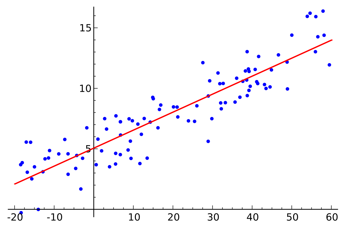
Linear regression is often thought of as a “straight line fit” to a set of observations. It doesn’t necessarily result in a straight line or flat plane, though. Consider that the “true” relationship or “population regression line” between $ Y \in \mathbb{R}^{m \times 1} $ (the response values associated with each row/observation of $ \mathbf{X} $) and $ \mathbf{X} $ is

$$ Y = f(\mathbf{X}) + \epsilon = \mathbf{X}\beta + \epsilon $$

Epsilon ($ \epsilon $) here represents the error term, encompassing omitted and unmeasurable predictors, measurement error of included predictors, and the generic inability of our selected linear model to fit the true relationship.

Indicators that Linear Regression Model is Lacking

After coming up with a linear regression model, there are various required checks in order to validate that the model is acceptable as a description of the data. If any of the following are true, it is necessary to either improve the data, model or accept linear regression is insufficient as a modeling technique under the given conditions.

Non-linearity of the response-predictor relationships

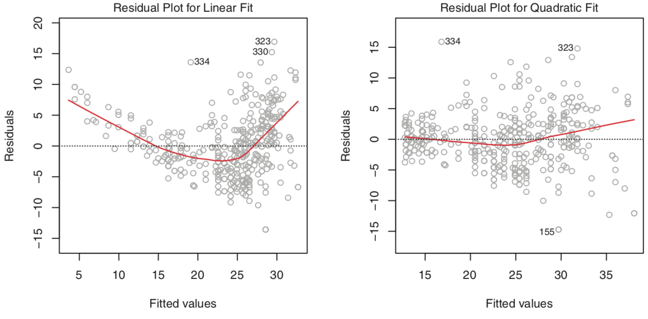
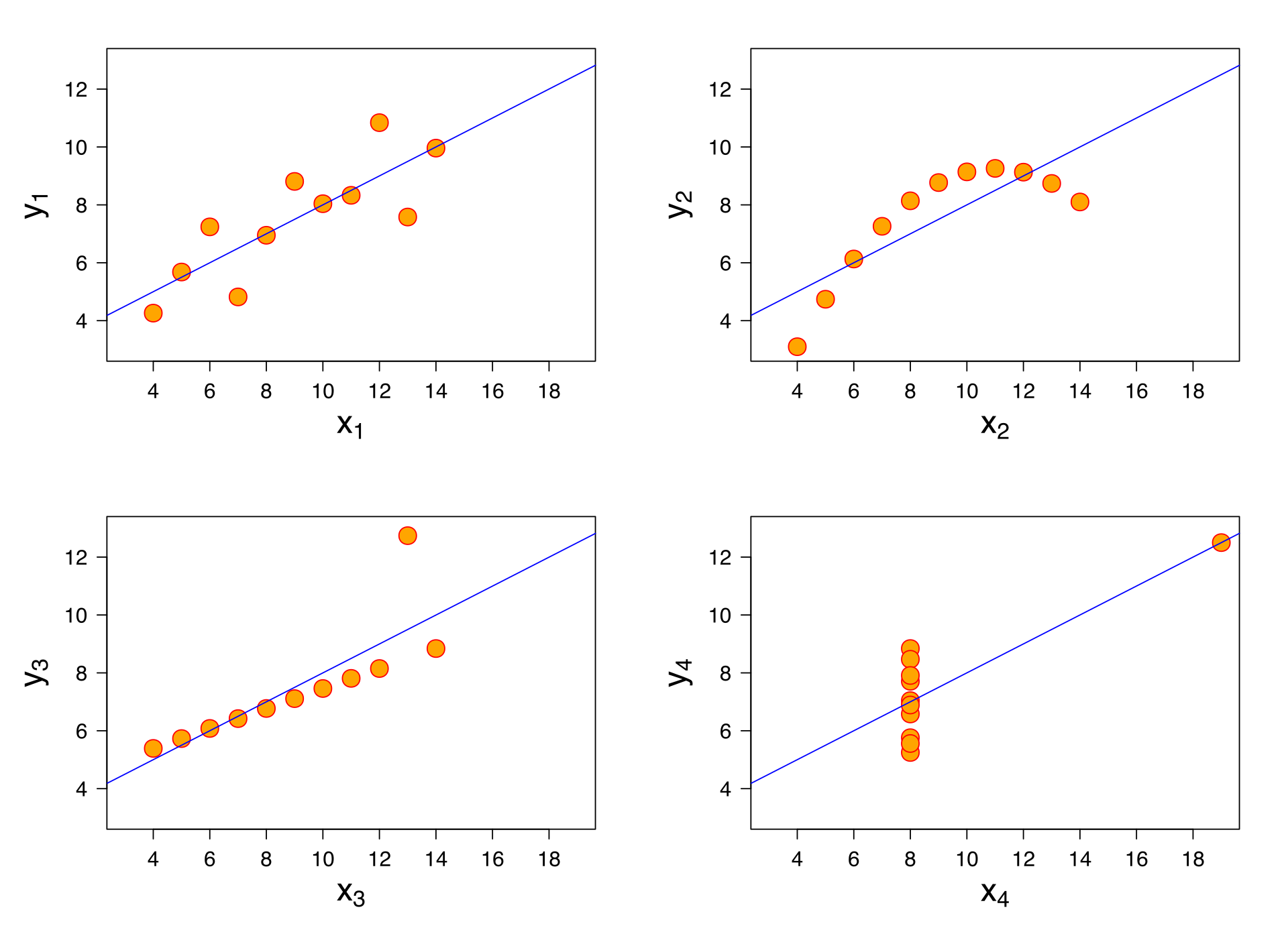
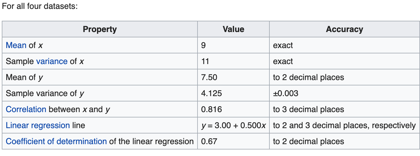
Left plot shows trend in residuals while right plot indicates better fit

There should be a linear relationship between the predictors and the response. This can be confirmed or denied by plotting the residuals $ e_i = y_i - \hat{y}_i $ versus the fitted values $ \hat{y}_i $. If the residuals look evenly dispersed about the horizontal access, the model is reasonable. Note that a poor residual plot may just be an indicator of poor predictor selection, e.g. non-linear predictors ($ x^2, \sqrt{x} $, etc.) should be fed in to the model.

Correlation of error terms

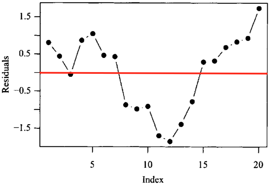
Correlated errors: adjacent errors tend to be of similar sign and magnitude

Given ordered data (e.g. time series), plot the residuals in order of time. If patterns arise, it is likely your data has correlated error terms. In time series data, this is also called autocorrelation. This could occur, for example, if you duplicated your time series dataset - looking at error terms in order, each one would have perfect correlation with the next or previous value! You would get the same parameter fits but drastically different confidence bounds. Other real world examples include sampling biological metrics from the same family or the stock market doing well during certain time periods and poorly in others. At times adding predictors to the model can solve this problem. There are also techniques for removal of autocorrelation with transformation.

Non-constant variance of error terms

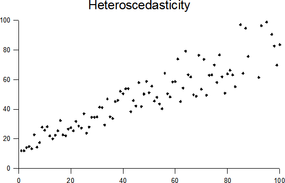
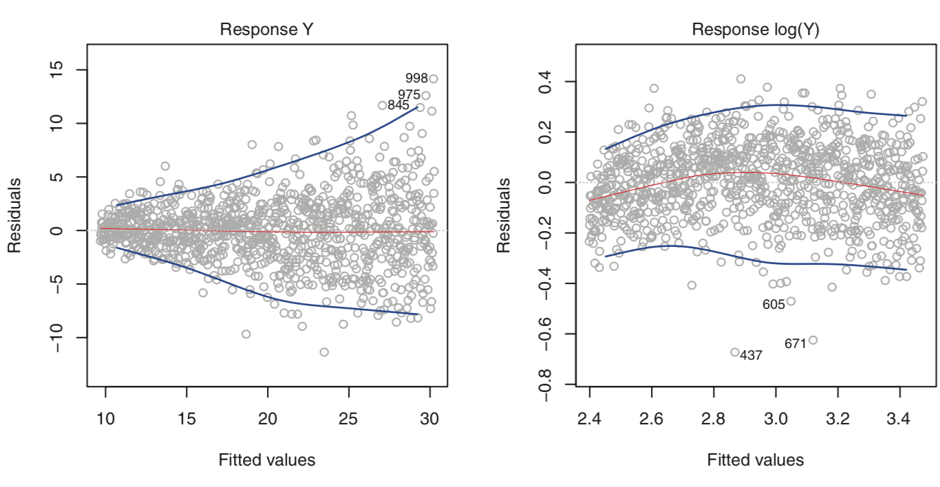
Heteroscedasticity can sometimes be removed by transforming the response

For linear regression’s standard errors, confidence bounds, and hypothesis tests, it is assumed that data was generated from a population regression line where the true error $ \epsilon $ is normally distributed with mean 0 and constant variance $ \sigma^2 $, that is $ \epsilon \sim N(0, \sigma^2) $. In reality, it is often the case in that $ \sigma^2 $ varies with the magnitude of the predictors and/or response - this is called heteroscedasticity. Transformation of the response may help the situation. If you have an idea of the variance of error at each response, you can also use weighted least squares.

Data contain outliers

Outlier points have abnormally high residuals. Methods exist for determining what “abnormal” means here, including examining the studentized residuals (dividing residuals by their estimated standard error). Outliers may not dramatically affect the weights of a model, but can affect the confidence bounds, hypothesis tests and $ R^2 $ value. Removing outliers is sometimes favorable, especially if they stem from something like measurement error. Before removal, it’s important to be sure that outliers aren’t actually important pieces of data implying that your model is missing predictors or is somehow otherwise deficient.

Data contain high-leverage points

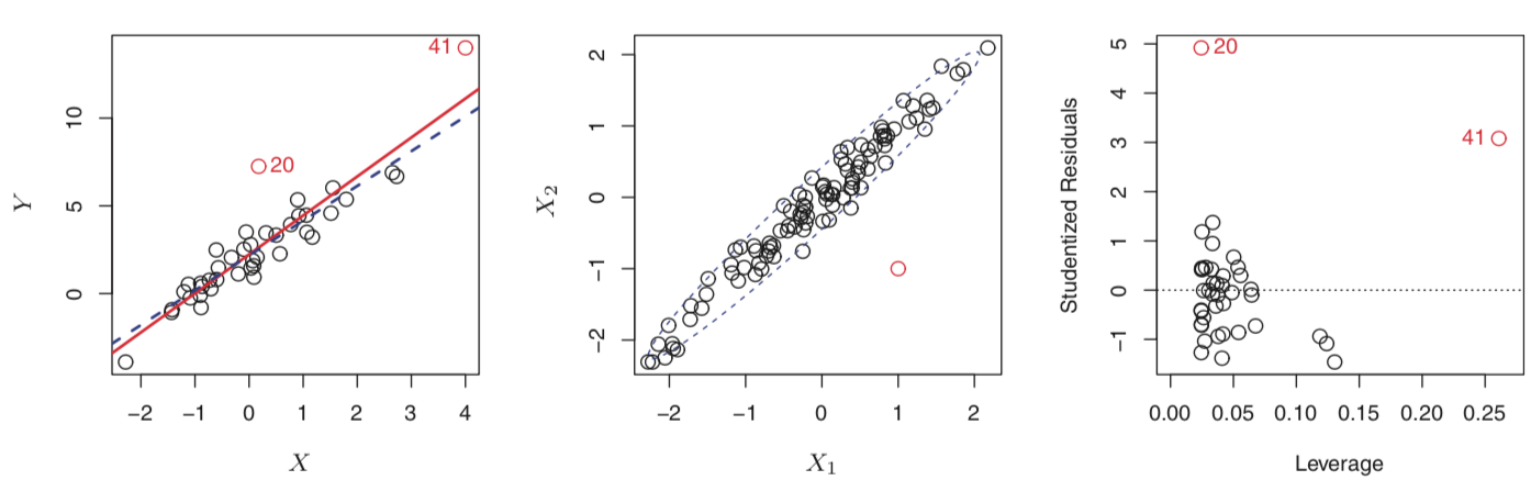
Leverage: not just for negotiation anymore

High leverage points have unusual predictor values, e.g. point 41 on the left plot above. Note that in multiple regression it can appear that high leverage points appear normal if you only examine each predictor value individually (middle graph above). Instead, calculate leverage using the diagonal of the “projection matrix” $ \mathbf{H} = \mathbf{X}(\mathbf{X}^T\mathbf{X})^{-1}\mathbf{X}^T $. Methods for determining what leverage magnitude is unusual enough to be suspect exist, including the Williams Graph similar the rightmost plot above.

Collinearity

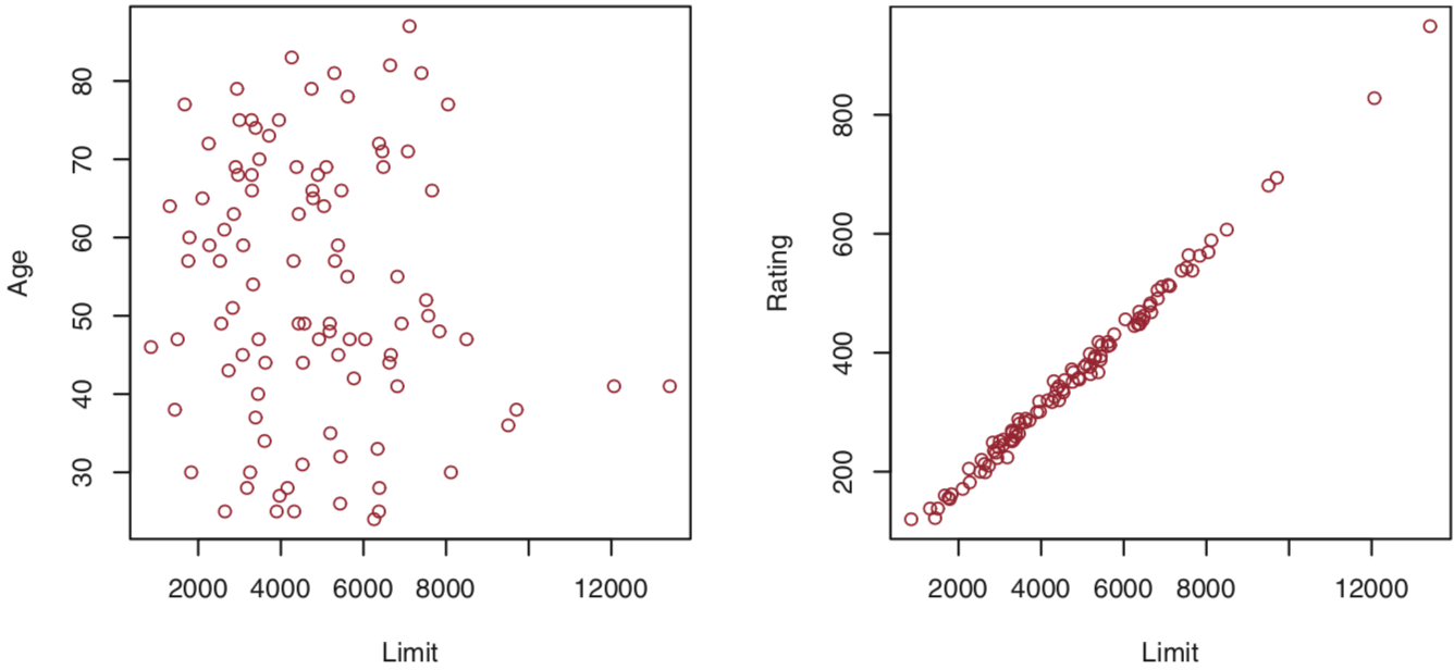
Age and limit are not collinear while rating and limit are highly collinear

Collinearity occurs when 2 or more predictors are highly related. This reduces the accuracy of the estimates of the weights, as it becomes hard to parse out which predictor is having an effect on the response. Detecting collinearity can be done by calculating the Variance Inflation Factor, and solved by either removing one of the collinear predictors or combining collinear predictors together.

Endogeneity

Endogeneity occurs when there is correlation between model predictor(s) and the true error term $ \epsilon $. Note that the error term here is NOT the estimated error term $ \hat{\epsilon} $ as a result of the fitted values $ \hat{Y} $, but the true error term in the population regression line $ Y = \mathbf{X}\beta + \epsilon $. An example I found explained it well was the burger regression here. Upon suspicion that a predictor is endogenous, a way to test for it is outlined here. Enogeneity is different than heteroscedasticity, as explained here.

Notes on $ R^2 $ (coefficient of determination)

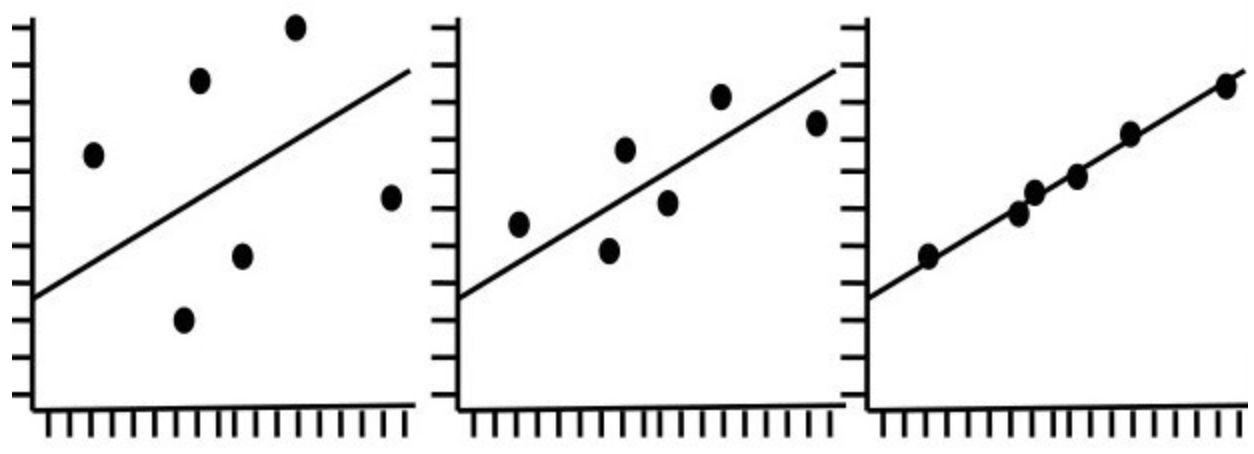
$ R^2 $ does nothing except measure the proportion of variability in Y that can be explained using X. It can always be made closer to 1 by adding more features/variables into the linear model, which at a certain point likely results in a too-flexible (overfit) model that fails to minimize test error. Where $ R^2 $ can be useful is in confirming previously held beliefs about what you are modeling. For example, modeling something in physics that theoretically should be extremely linear, an $ R^2 $ much smaller than 1 indicates something may be off with the model or data. Conversely, a low $ R^2 $ would actually be expected when modeling a complex situation with high residual errors due to other factors.

Normal Equation for Estimated Weights $ \hat{\beta} $

In the Ordinary Least Squares approach, RSS (Residual Sum of Squares) as a function of $ \hat{\beta} $ is the function to minimize:

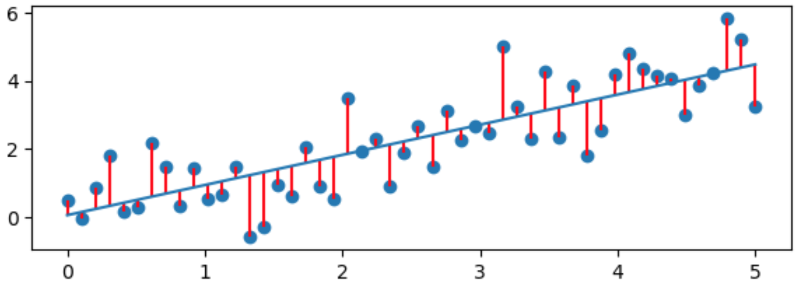
Red lines are residuals $ e_i $. RSS is the sum of the square of all residuals

$$RSS = \sum_{i=1}^{m}e_i^2 = \sum_{i=1}^{m}(y_i - \hat{y_i})^2 = \sum_{i=1}^{m}(y_i - x_i^T\hat{\beta})^2$$ where $y_i$ is the response and $\hat{y}_i = x_i^T\hat{\beta}$ is the fitted value. This is assuming $x_i \in \mathbb{R}^{n \times 1}$ and $\hat{\beta} \in \mathbb{R}^{n \times 1}$ are column vectors and that the first value in each $ x_i $ is 1.

We can rewrite this in matrix form with $\bf{X} \in \mathbb{R}^{m \times n}$ and $y \in \mathbb{R}^{m \times 1}$ as $$RSS(\hat{\beta})=(y - \mathbf{X}\hat{\beta})^T(y - \mathbf{X}\hat{\beta})$$

Each estimated weight vector $\hat{\beta}$ will give a different $RSS$ value. Since the premise of Ordinary Least Squares (OLS) is minimizing $RSS$, we can take the derivative of $RSS(\hat{\beta})$ and set it to zero to obtain the normal equations for the $\hat{\beta}$ that minimizes $RSS$. Note that we use $ (\mathbf{AB})^T = \mathbf{B}^T\mathbf{A}^T $ and the fact that matrices are distributive: $$RSS(\hat{\beta})=(y^T - (\mathbf{X}\hat{\beta})^T)(y - \mathbf{X}\hat{\beta})$$ $$RSS(\hat{\beta})=(y^T - (\hat{\beta}^T\mathbf{X}^T))(y - \mathbf{X}\hat{\beta})$$ $$RSS(\hat{\beta})=y^Ty - y^T\mathbf{X}\hat{\beta} - (\hat{\beta}^T\mathbf{X}^T)y + \hat{\beta}^T\mathbf{X}^T\mathbf{X}\hat{\beta}$$

Taking the derivative with respect to the estimated weights: $$ \frac{\partial}{\partial{\hat{\beta}}}RSS(\hat{\beta}) = $$ $$ \color{grey}{\frac{\partial}{\partial{\hat{\beta}}}y^Ty} \color{black}{-} \color{red}{\frac{\partial}{\partial{\hat{\beta}}}(y^T\mathbf{X}\hat{\beta} + (\hat{\beta}^T\mathbf{X}^T)y)} \color{black}{+} \color{green}{\frac{\partial}{\partial{\hat{\beta}}}\hat{\beta}^T\mathbf{X}^T\mathbf{X}\hat{\beta}} $$

Now luckily, $\color{grey}{\frac{\partial}{\partial{\hat{\beta}}}y^Ty}=0$ as response $y$ is independent of $\hat{\beta}$. In addition, the red term isn’t so bad. Because $RSS$ is scalar, each term is a scalar. And since scalars are symmetric, $a^T=a$. Again, we use $ (\mathbf{AB})^T = \mathbf{B}^T\mathbf{A}^T $.

So the following holds: $$\color{red}{ \frac{\partial}{\partial{\hat{\beta}}} (y^T\mathbf{X}\hat{\beta} + (\hat{\beta}^T\mathbf{X}^T)y) }$$ $$\color{red}{ = \frac{\partial}{\partial{\hat{\beta}}} ((y^T\mathbf{X}\hat{\beta})^T + (\hat{\beta}^T\mathbf{X}^T) y) }$$ $$\color{red}{ = \frac{\partial}{\partial{\hat{\beta}}} ((\mathbf{X}\hat{\beta})^Ty + (\hat{\beta}^T\mathbf{X}^T)y) }$$ $$\color{red}{ = \frac{\partial}{\partial{\hat{\beta}}} ((\hat{\beta}^T\mathbf{X}^T)y + (\hat{\beta}^T\mathbf{X}^T) y) }$$ $$\color{red}{ = \frac{\partial}{\partial{\hat{\beta}}} 2\hat{\beta}^T\mathbf{X}^Ty }$$

We can take advantage of the “A is not a function of x” identity here, $ \frac{\partial{x^T\mathbf{A}}}{\partial{x}} = \mathbf{A} $. There is a great intuitive walkthrough of this identity here if interested. $$\color{red} {2\frac{\partial\hat{\beta}^T\mathbf{X}^Ty}{\partial{\hat{\beta}}} = 2\mathbf{X}^Ty }$$

The green term uses another identity, “A is not a function of x, A is symmetric” here, $ \frac{\partial{x^T\mathbf{A}x}}{\partial{x}} = 2\mathbf{A}x $. Note that this relies on the $ \mathbf{A} $ matrix being symmetric, but since $ \mathbf{X}^T\mathbf{X} $ is indeed symmetric, this holds. Again, there is a great intuitive walkthrough of this other identity here if interested as well. $$ \color{green} {\frac{\partial\hat{\beta}^T\mathbf{X}^T\mathbf{X}\hat{\beta}}{\partial{\hat{\beta}}} = 2\mathbf{X}^T\mathbf{X}\hat{\beta} }$$

Finally, we plug in all terms and set to 0: $$ \frac{\partial}{\partial{\hat{\beta}}}RSS(\hat{\beta}) = \color{grey}{0} \color{black}{-} \color{red}{2\mathbf{X}^Ty} \color{black}{+} \color{green}{2\mathbf{X}^T\mathbf{X}\hat{\beta}} \color{black}{\ = 0} $$

Rearranging, we get: $$ \color{red}{\mathbf{X}^Ty} \color{black}{=} \color{green}{\mathbf{X}^T\mathbf{X}\hat{\beta}} $$

And if $ \mathbf{X}^T\mathbf{X} $ is nonsingular, i.e. it has an inverse, we can solve directly for $ \hat{\beta} $ using the following: $$ \hat{\beta} = (\mathbf{X}^T\mathbf{X})^{-1}\mathbf{X}^Ty$$

This is called the normal equation. It is helpful when the inverse $ (\mathbf{X}^T\mathbf{X})^{-1}\ $ is not too computationally intensive.

Maximum Likelihood Estimate Formulation

From wikipedia: “Maximum Likelihood Estimation is a method of estimating the parameters of a probability distribution by maximizing a likelihood function, so that under the assumed statistical model the observed data is most probable”. Some probabilistic process generated some data - which process parameters would have made our dataset the most likely? Expressed as conditional probability distributions, for some data, which parameters maximize $ P(data | parameters) $?

As stated before, the population regression line is:

$$ Y = \mathbf{X}\beta + \epsilon $$

where $ \mathbf{X}\beta $ is constant. Gaussian linear regression assumes that $ \epsilon $ is normally distributed with mean 0 and variance $ \sigma^2 $, $ \epsilon \sim N(0, \sigma^2) $. Examining the distribution of $ Y$ under this assumption, noting that $E[X + Y] = E[X] + E[Y] $ regardless of independence:

$$ E[Y] = E[\mathbf{X}\beta + \epsilon] $$ $$ = E[\mathbf{X}\beta] + E[\epsilon] $$ $$ = E[\mathbf{X}\beta] + 0 $$ $$ = \mathbf{X}\beta $$

And for variance, since

$$ Var(X) = E[X^2] - (E[X])^2 $$

from here and

$$ Cov(X,Y) = E[XY] - E[X]E[Y] $$

from here, then:

$$ Var(A + B) = E[(A + B)^2] - (E[A + B])^2 $$ $$ = E[A^2 + 2AB + B^2] - (E[A] + E[B])^2 $$ $$ = E[A^2] + E[2AB] + E[B^2] $$ $$ - E[A]^2 - 2E[A]E[B] - E[B]^2 $$ $$ = E[A^2] - E[A]^2 $$ $$ + E[B^2] - E[B]^2 $$ $$ + 2(E[AB] - E[A]E[B]) $$ $$ = Var(A) + Var(B) + 2Cov(A,B) $$

Substituting $A = \mathbf{X}\beta $, $B = \epsilon$ and recognizing Covariance as a measure of correlation between variables - positive if both tend to increase together, negative when one tends to increase while the other decreases - we can say:

$$ Var(\mathbf{X}\beta + \epsilon) = Var(\mathbf{X}\beta) + Var(\epsilon) + 2Cov(\mathbf{X}\beta, \epsilon) $$ $$ = 0 + \sigma^2 + 2Cov(\mathbf{X}\beta, \epsilon) $$

Due to the assumptions of linear regression outlined above (exogeneity and homoscedasticity), the correlation between $\mathbf{X}\beta$ and $\epsilon$ is zero. We conclude:

$$ Var(Y) = \sigma^2 $$

so:

$$ Y \sim N(\mathbf{X}\beta, \sigma^2) $$

With this in mind, we begin the actual MLE derivation. Given that the PDF of the gaussian distribution is:

$$ P(x|\mu_x, \sigma_x^2) = \frac{1}{\sigma_x\sqrt{2\pi}} \exp{\left\lbrace-\frac{1}{2\sigma_x^2}(x-\mu_x) \right\rbrace} $$

we can say the conditional probability of some datum $ y_i $ based on our parameters is:

$$ P(y_i|x_i, \beta, \sigma^2) = \frac{1}{\sigma\sqrt{2\pi}} \exp{\left\lbrace-\frac{1}{2\sigma^2}(y_i - x_i\beta) ^2\right\rbrace} $$

where we somehow go through $ i = 0,1,2,…m $ data points and obtain the joint probability of all of them. Assuming our data are i.i.d. (independently and identically distributed, i.e. sampled from the same probability distribution and independent of one another) - we can say the joint probability of all the data is a product of individual probabilities:

$$ P(\{y_i\}_{i=0}^m | \{x_i\}_{i=0}^m, \beta, \sigma^2) = $$ $$ \prod_{i=0}^m{\frac{1}{\sigma\sqrt{2\pi}} \exp{\left\lbrace-\frac{1}{2\sigma^2}(y_i - x_i\beta)^2\right\rbrace}} $$

In matrix form: $$ P(Y|X,\beta,\sigma^2) = $$ $$ \left(\frac{1}{\sigma\sqrt{2\pi}}\right)^m \exp{\left\lbrace-\frac{1}{2\sigma^2}(y-\mathbf{X}\beta)^T( y-\mathbf{X}\beta)\right\rbrace} $$

With MLE, we often take the log, as maximizing a summation is easier than maximizing a product due to ease of derivation. Note that the parameters that maximize some random variable X are the same that maximize log(X), so we’re ok doing this. $$ \ln(P(Y|X,\beta,\sigma^2)) = $$ $$ \color{red}{ m\ln\left(\frac{1}{\sigma\sqrt{2\pi}}\right) } \color{black}{ - } \color{green}{ \frac{1}{2\sigma^2}(y-\mathbf{X}\beta)^T(y-\mathbf{X}\beta) } $$

Note that the red term doesn’t have a $ \beta $ and is therefore irrelevant while we try to find the $ \beta $ that maximimizes $ \ln(P(Y|X,\beta,\sigma^2)) $. In order to do this, we must actually MINIMIZE the green term, as it’s negative! So let’s see…we want to minimize… $$ \frac{1}{2\sigma^2}(y-\mathbf{X}\beta)^T(y-\mathbf{X}\beta) $$

Sound familiar? It’s the same problem as the “Normal Equation for Estimated Weights” section before! This will again result in the normal equation: $$ \beta^{MLE} = (\mathbf{X}^T\mathbf{X})^{-1}\mathbf{X}^Ty$$

Now note, we ignored the red term above to get the $ \beta^{MLE} $, but we can also maximize the joint probability distribution with respect to $ \sigma^2 $ in the MLE formulation. We derive and set to zero to find the maximum: $$ \frac{\partial}{\partial{\sigma}} \left( \color{red}{ m\ln\left(\frac{1}{\sigma\sqrt{2\pi}}\right) } \right) \color{black}{ - \frac{\partial}{\partial{\sigma}} } \left( \color{green}{ \frac{1}{2\sigma^2}(y-\mathbf{X}\beta)^T(y-\mathbf{X}\beta)) } \right) $$ $$ = \color{red}{ -m (\sigma\sqrt{2\pi}) \left(\frac{1}{\sigma^2\sqrt{2\pi}}\right) } \color{black}{ + } \color{green}{ \frac{1}{\sigma^3}(y-\mathbf{X}\beta)^T(y-\mathbf{X}\beta)) } $$ $$ = \color{red}{ -m } \color{black}{ + } \color{green}{ \frac{1}{\sigma^2}(y-\mathbf{X}\beta)^T(y-\mathbf{X}\beta)) } \color{black}{ = 0 } $$

Rerranging, we get the MLE estimate for the variance of $ \epsilon $: $$ \sigma^{2MLE} = \frac{1}{m}(y-\mathbf{X}\beta)^T(y-\mathbf{X}\beta) $$

And note how this (satisfyingly) resembles the population variance formula for a normal distribution: $$ \sigma^2_x = E[(x - \mu_x)^2] $$

Confidence in Estimated Parameters

(Insert justification for searching for unbiased sigma^2 and variance of beta in the first place here)

Unfortunately, the MLE variance is actually a biased estimate of the population variance, i.e. $ E[\sigma^{2MLE}] \neq \sigma^2 $! For a discussion around this and empirical proof, see here.

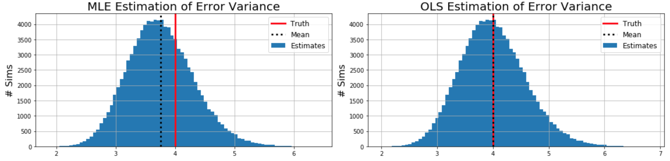
MLE (left) mean estimate differs from the true value

The unbiased formula for estimated error variance comes from here and the rigorous proof here: $$ \sigma^{2OLS} = \frac{1}{m-n} (y-\mathbf{X}\beta)^T (y-\mathbf{X}\beta) $$

(Variance of beta here)

To be included sometime in the future: standard errors, confidence bounds, hypothesis tests, numerical methods.