statistical bias

Oct 25, 2019

You find yourself trapped in a room with Jigsaw, the villain from the Saw movies. There is a wood box of 100 spheres, some of them steel ball bearings and some of them gumballs. Jigsaw tells you that you can leave the room alive if you guess the number of steel ball bearings in the jar correctly. You can pull 10 random spheres out the 100 in the box as many times as you want, but each time you do, you have to eat all of them (yum!). Jigsaw will then replace the stuff you pulled out of the box with new ones - if you pulled 7 ball bearings and 3 gumballs, 7 and 3 are replaced respectively. You’re like “cool, I got this, I’m just going to do this a bunch of times and average the number of ball bearings I have to eat each time, then multiply the average by 10 and go home to my family of 12”. Little did you know, Jigsaw has implanted magnets in your fingertips, attracting the ball bearings. Your estimate will be biased no matter how many spheres you eat. You will be killed, and your family will mourn.

Bias, both in common vernacular and in statistics, can be thought of as the difference between the average estimate of some truth and the truth itself. Your cousin is biased because his opinions on the evils of gun control, while varied, are on average far from the truth. A statistical model is biased because the average difference between its fitted and true values are non-zero.

Say you estimate a model parameter, e.g. $ \hat{\beta} $, based off a sample of data. Assuming the data comes from some underlying distribution with true parameter $ \beta $, your estimate $ \hat{\beta} $ is unbiased if the average estimate of it is equal to the true parameter, i.e. $ E[\hat{\beta}] = \beta $.

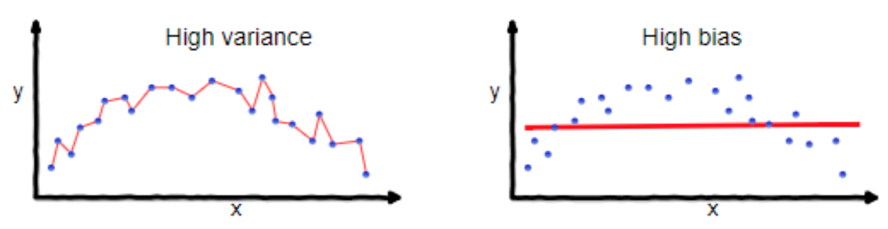
The concept of bias-variance tradeoff is fundamental in modeling. Intuitively, bias is the average difference in model prediction to true value, as discussed above. Variance is how much the model changes when you alter the sample data.

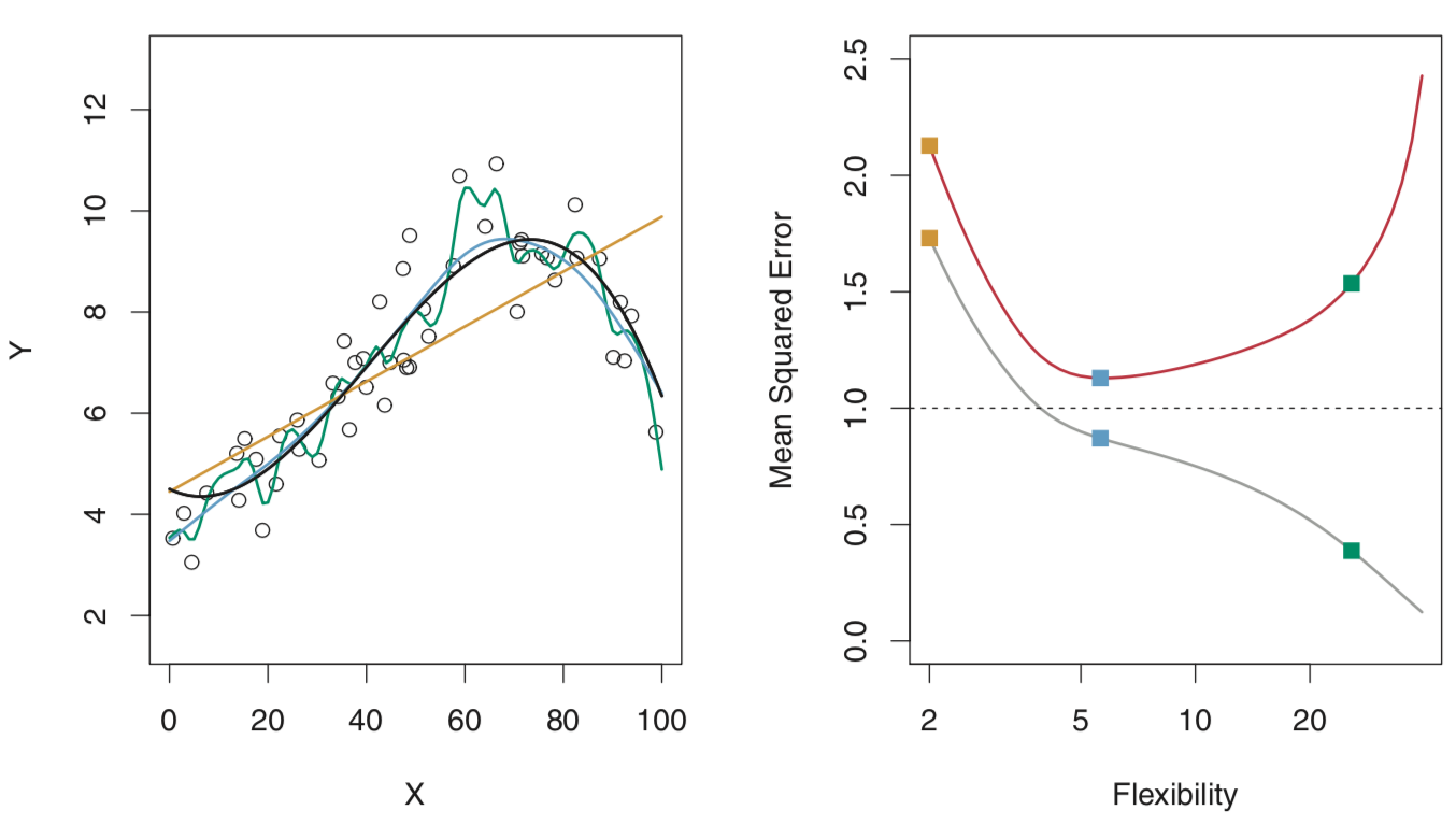
Say, theoretically, that your goal is to have a good model. You might say “I want my model’s predictions to be close to reality”. Even, “I want the average squared-error of my models predictions to be minimized!”. That’s not a bad idea! But wait - the image on the left above looks great for that, right? Why is that not the best model? Because the points that this model is going through don’t represent all the possible points - it’s just a data sample. If you got some more data, your model might not perform very well - its mean-squared error (MSE) might go up.

Demonstrated visually, 3 models fit the data below. They increase in number of predictors, i.e. flexibility of the model. Note how there is always some model error (dashed line on right) - this is the irreducible error, due to things like randomness in the generation of future data and inability to parameterize the universe. The red line represents our test error, our test set being some data we withheld from the model while estimating its parameters. The grey line represents the training error, based on the data we estimated our model parameters with. Training error CAN go to zero, as in the left image above, but we really care about our test error. Test error represents our model’s ability to make accurate future predictions.

Note that MSE can be mathematically decomposed in to bias and variance terms. Assume for some data sample/training set, it came from same “data generating function” $y = f(x) + \epsilon $ where $ \epsilon \sim N(0, \sigma^2) $. We want to find the $ \hat{f}(x) $ that results in predictions for $ y $ that minimize MSE for data even outside our sample.

$$ E[(y - \hat{f}(x))^2] = MSE $$ $$ = Bias[\hat{f}(x)]^2 + Var(\hat{f}(x)) + \sigma^2 $$

Proofs for this exist here and here.

The bias-variance tradeoff has an important consequence: it is possible that an increase in bias can actually decrease variance to the point where overall MSE is better! A good model minimizes MSE, not just bias or variance.

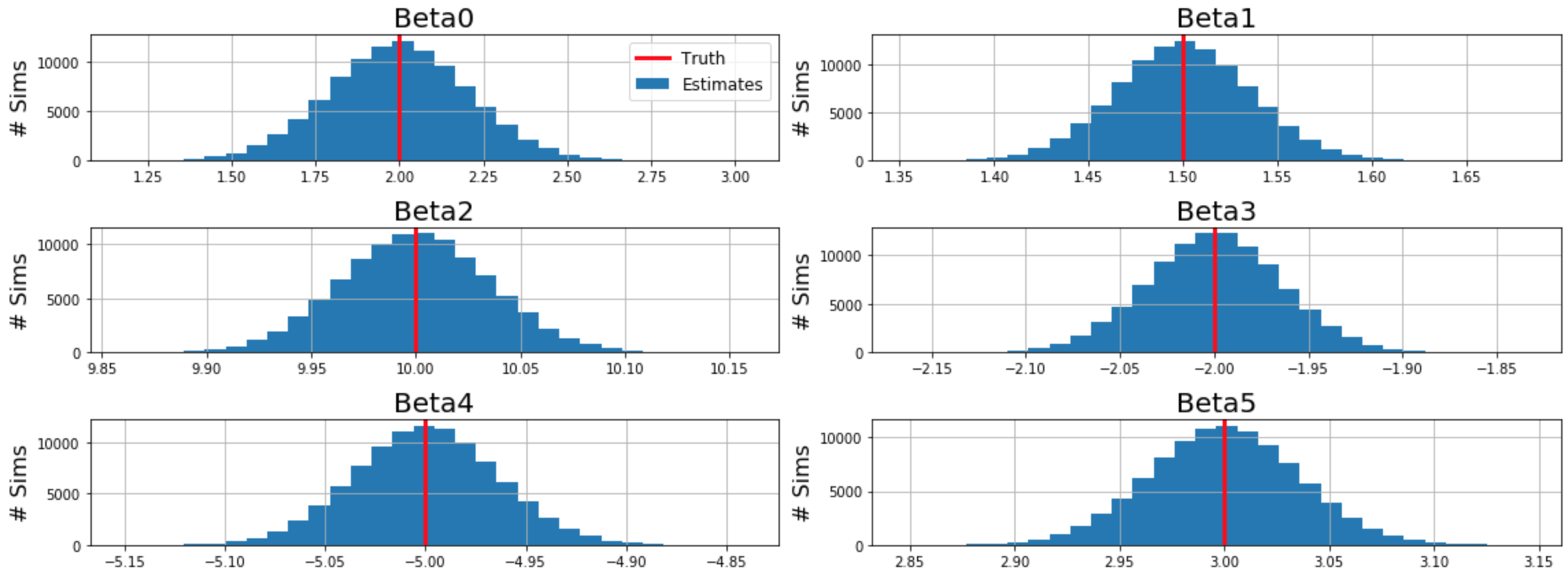
A concrete example of biased estimators exists below. Generating many samples from an underlying function, both MLE and OLS methods result in unbiased estimates of weights:

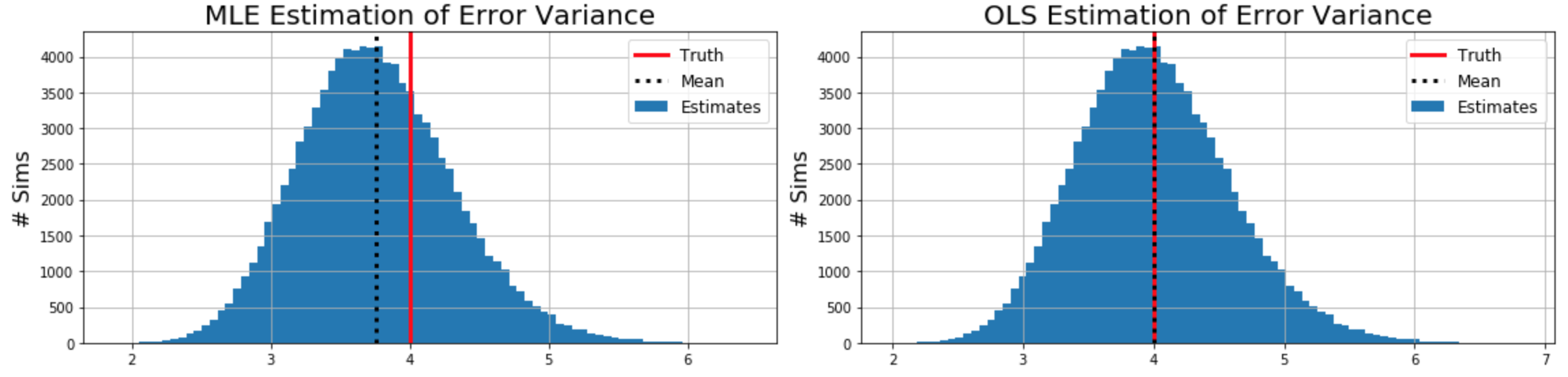
The mean estimate for each weight is the same as the red true value

Importantly, the MLE estimate for error variance $ \sigma^2 $ is biased, whereas the OLS estimate is unbiased. Note that the only difference between the MLE and OLS estimates is dividing by $ m - n $, the number of samples minus the number of predictors. Some intuition for how sample variance is biased without this division can be built from this proof, while a more involved proof of the unbiased OLS error variance formula lies here.

MLE (left) mean estimate differs from the true value

Complete code for the simulation can be found in the static notebook here.

I hope this helped develop a deeper understanding of statistical bias. If you have any additions or errors to correct, please open an issue on the source of this website here.

statistical bias

References: